34
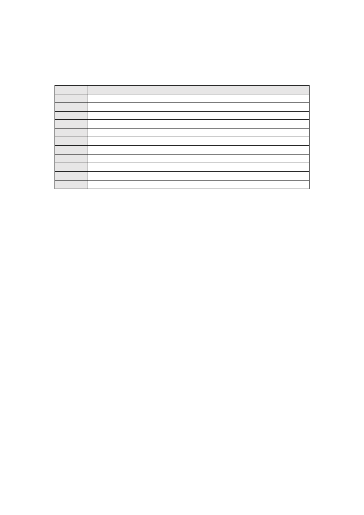
The difference between the ratio of REJ and S0 flags, which are the most prominent after the
SF flag, can be understood after looking at what each label means, in Table 4:
Table 4: flags in the NSL-KDD dataset
Name
Meaning
SF
Normal establishment and termination
S0
Connection attempt, no reply
REJ
Connection attempt rejected
RSTR
Connection reset by the destination
RSTO
Connection reset by the source
S1
Connection establishment, no termination
SH
Source sent a SYN and FIN, without a SYN-ACK from the destination
S2
Connection established, close attempt from source but no reply
RSTOS0
Source sent a SYN and RST, without a SYN-ACK from the destination
S3
Connection established, close attempt by destination but no reply
OTH
No SYN, just midstream traffic that is not later closed
In the test set, where the abnormal traffic is higher, it is natural to have more rejection flags,
whereas in the training set, where the normal traffic prevails, more connection attempts are
to be expected.
4.3. Pre-processing of the NSL-KDD dataset
One of the most important steps in creating a data science model is pre-processing the data.
Python is a language especially capable of handling tasks that have to do with data handling
and processing, and in this section, the preparation of the dataset is going to be described step
by step. Essentially, the dataset was imported to a Jupyter notebook as a dataframe, the
categorical variables were encoded as numerical ones, and the data was scaled so that it didn’t
bias the importance of each feature.
Firstly, the NSL-KDD dataset, as a set of .csv files (KDDTrain+ and KDDTest+), was loaded into
the notebook by using the pandas library. Pandas is a crucial library for most of the operations
done on the data, from reading/writing, to handling the dataset column by column and
encoding it.
Using pandas, the dataset was loaded into two dataframe type variables, one for the training
and one for the testing subset. Their lengths are 125,973 and 22,544 records respectively,
and they both have 43 columns (0 − 42).
Other than the two multiclass datasets (Figure 18), two more pairs of training – test dataframes
were created, one for binary classification (Figure 19), where #42 labels were turned into
‘normal’ and ‘abnormal’, and one for the 4-class classification (Figure
), where #42 labels
were turned into ‘normal’, ‘DoS’, ‘Probe’, ‘R2L’ and ‘U2R’ labels.