19 

 

The  variable  𝑧  describes  the  input  value,  which  is  the  variables  vector  of  the  entries  𝑋

𝑖

=

{𝑥

0

, 𝑥

1

, … , 𝑥

𝑛−1

} (for 𝑛 number of features in the dataset) multiplied by weight values, that 

will be tweaked as the model tries to predict 𝑦 with respect to 𝑋

𝑖

. 

𝑦(𝑥) = 𝜃

0

𝑥

0

+ 𝜃

1

𝑥

1

+ ⋯ + 𝜃

𝑛−1

𝑥

𝑛−1

= ∑ 𝜃

𝑖

𝑥

𝑖

𝑛−1

𝑖=0

= 𝜃

𝑇

𝑋 

Equation 2: output y as a function of the input values X 

Thus, in the case of logistic regression, this abstract function becomes 𝑦 = 𝑔(𝜃

𝑇

𝑋

𝑖

). Through 

the training of the model, the weight values (𝜃

𝑡

) are randomly initialized and then change so 

that the loss function is minimized, and this sets the threshold for which 𝑦 = 1 or 𝑦 = 0. 

Logistic regression is one of the simplest machine learning algorithms, so it doesn’t need many 
conditions to generate satisfactory results and doesn’t require much CPU power usually. It also 
doesn’t  overfit  as  much as  more  complex  algorithms  and  can  easily  update  with  new  data. 
Nevertheless, its simplicity hinders its performance on higher dimension datasets, and highly 
correlated variables in a dataset should be avoided; also, it needs to train with larger datasets 
without redundant records in them [15]. 

 

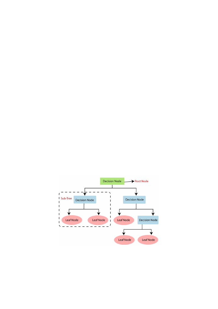
3.2. Decision Tree 

The decision tree classifier is a tree-shaped algorithm that is commonly used for classification 
applications.  

 

Figure 2: decision tree classifier representation (source 

[16]

) 

The root node represents the beginning of the decision tree and includes the whole dataset. It 
gets further divided (splitting) as the algorithm poses conditions to the dataset that create sub-
classes according to the outcome of each entry. Through the splitting process, branches are 
created,  as  different  classes  of  data  follow  different  paths.  The  leaf  nodes  represent  the